How You Lift Matters: Wearable Sensors Can Detect Exercise Form Errors with 99% Accuracy

machine learning

random forest

gradient boosting

decision tree

classification

lifting form

Author

Kara C. Hoover

Published

June 2021

Executive Summary

Problem: Fitness tracking technology typically measures whether people exercise but not how well they move. Poor exercise form is a leading cause of injury, yet wearable sensors are rarely used to distinguish correct technique from specific, identifiable mistakes in real time.

Approach: Accelerometer data from sensors strapped to participants’ belts, forearms, arms, and dumbbells were used to classify bicep curl form across five categories: one correct technique (Class A) and four defined errors (Classes B–E), including elbow flaring, incomplete range of motion, and excessive hip involvement. Four machine learning algorithms were compared – a decision tree, a bagged decision tree, a gradient boosted random forest, and a random forest – to identify which model best separates form classes and which sensor locations contribute most to accurate classification.

Insights: The random forest model achieved 99.4% accuracy with an out-of-sample error of just 0.6%, substantially outperforming the decision tree (49.7%) and demonstrating the power of ensemble methods for high-dimensional sensor classification. Accuracy peaked at 27 of 52 predictors rather than the full set, suggesting the model is over-parameterized and that a leaner deployment model is achievable with domain-informed feature selection.

Significance: As wearable fitness technology becomes more accessible, the ability to classify movement quality – not just movement quantity – opens the door to real-time coaching and injury prevention at scale. This project shows that a single well-tuned ensemble model can reliably distinguish between correct form and specific movement errors, which has direct application in consumer fitness devices and physical rehabilitation monitoring.

Key Findings

The random forest model achieved 99.4% accuracy (95% CI: 99.2–99.5%) with a Kappa of 0.992, correctly classifying all five form categories.
The decision tree performed at chance (49.7% accuracy) and failed to predict Class D (half-range lifting) entirely – a failure resolved completely by the random forest.
Resampling methods consistently outperformed the single decision tree: the bagged tree reached 95.8% accuracy and the gradient boosted forest reached 96.3%.
Model accuracy peaked at 27 predictors and declined at the full 52, indicating potential collinearity and a clear opportunity for feature reduction.
Sensor location and predictor importance varied across models, suggesting that a minimal sensor deployment (fewer than four body locations) may be sufficient for accurate classification.

Applied Findings

Ensemble methods – particularly random forests – are substantially more effective than single decision trees for classifying multi-class movement data from wearable sensors.
A production-ready wearable form classifier could be built on approximately half the current predictor set; domain expertise in exercise physiology should guide final feature selection.
Collinearity analysis is a recommended next step before any model deployment to avoid falsely inflated accuracy estimates.

Research Question

Can wearable accelerometer sensors reliably distinguish between correct exercise form and specific, defined technique errors during bicep curls – and if so, which sensor locations and model types provide the most accurate classification?

Research Answers

The core question was whether machine learning models could differentiate not just whether someone exercised, but how well they moved. The answer depends entirely on the model chosen: a single decision tree cannot solve this problem, but ensemble methods can. Results across all four models are summarized in Table 9 at the end of this section.

Decision Tree: Chance-Level Performance

The rpart decision tree achieved 49.7% accuracy (95% CI: 48.6–50.9%, Kappa: 0.343) – statistically indistinguishable from random guessing. Its most critical failure, visible in Table 1, was a complete inability to predict Class D (half-range lifting): every one of the 1,286 Class D observations was misclassified, with 577 assigned to A, 244 to B, and 465 to C. Table 2 confirms the consequence – sensitivity for Class D is undefined (NA) and prevalence records as zero, meaning the model never once predicted this class. Classes B and C also showed weak sensitivity (0.508 and 0.334 respectively). Class E was the only class the model handled reliably (sensitivity: 0.992), likely because its distinctive hip-forward movement pattern produces sensor readings sufficiently different from the others. The model lacks the variance-reduction mechanisms needed to separate visually similar movement patterns.

Table 1. Confusion Matrix – Decision Tree (rpart)

	A	B	C	E
A	2032	41	154	5
B	624	525	369	0
C	646	33	689	0
D	577	244	465	0
E	211	191	383	657

Table 2. Performance Statistics by Class – Decision Tree (rpart)

Statistic	A	B	C	D	E
Sensitivity	0.497	0.508	0.334	NA	0.992
Specificity	0.947	0.854	0.883	0.836	0.891
Pos Pred Value	0.910	0.346	0.504	NA	0.456
Neg Pred Value	0.633	0.920	0.788	NA	0.999
Prevalence	0.521	0.132	0.263	0.000	0.084
Detection Rate	0.259	0.067	0.088	0.000	0.084
Detection Prevalence	0.284	0.193	0.174	0.164	0.184
Balanced Accuracy	0.722	0.681	0.609	NA	0.942

Resampling Recovers Performance: Bagged Tree

The bagged tree – which averages multiple models produced by resampling – reached 95.8% accuracy (95% CI: 95.4–96.3%, Kappa: 0.947) and successfully predicted all five classes, including Class D which the decision tree missed entirely. Variable importance for the bagged tree is computed per class, reflecting which predictors most strongly distinguish each form category from the others. Figure 1 shows that belt and forearm sensor readings dominate across all five classes, with pitch and roll measurements consistently appearing among the top predictors. The per-class structure reveals meaningful differences – Class D (half-range) and Class E (hip-forward) show distinct importance profiles compared to Classes A, B, and C, consistent with their biomechanical differences.

Figure 1. Variable Importance by Class – Bagged Tree

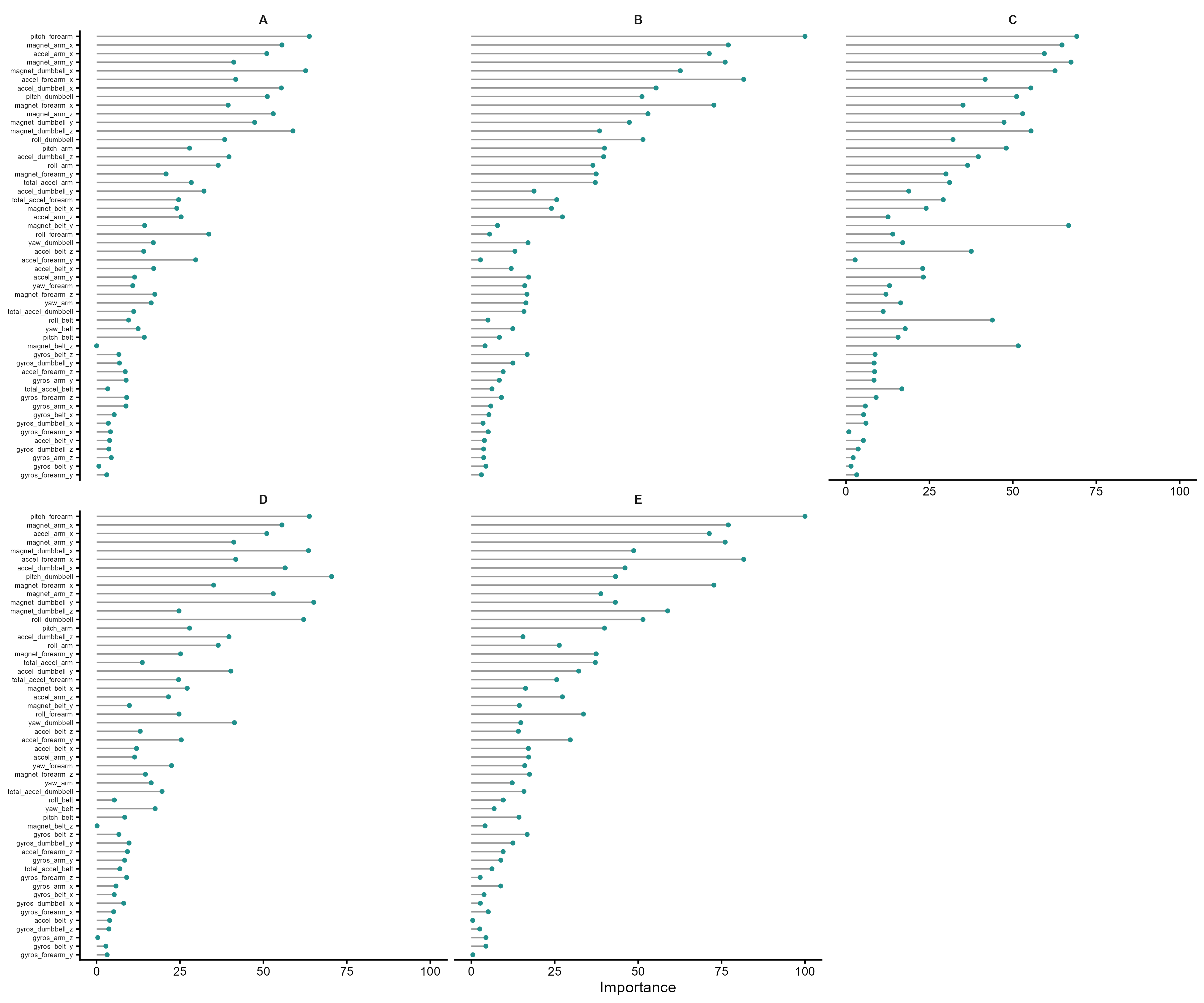
Interpretation: Belt and forearm sensors carry the most discriminating information across all five form classes. The class-by-class variation in importance profiles suggests that different movement errors activate different sensor signals – supporting the case for targeted sensor placement in any deployment scenario.

As shown in Table 3, misclassifications are now spread across the diagonal rather than collapsing into a few dominant classes – a dramatic improvement over rpart. Table 4 shows sensitivity ranging from 0.934 (Class C) to 0.982 (Class E), with specificity above 0.986 for all classes, indicating very few false positives in any category.

Table 3. Confusion Matrix – Bagged Tree

	A	B	C	D	E
A	2180	28	10	9	5
B	33	1429	47	11	18
C	2	36	1294	24	1
D	6	5	33	1231	11
E	5	9	13	22	1384

Table 4. Performance Statistics by Class – Bagged Tree

Statistic	A	B	C	D	E
Sensitivity	0.979	0.936	0.934	0.949	0.982
Specificity	0.991	0.986	0.989	0.992	0.991
Pos Pred Value	0.977	0.941	0.946	0.957	0.960
Neg Pred Value	0.992	0.985	0.986	0.990	0.996
Prevalence	0.284	0.195	0.177	0.165	0.180
Detection Rate	0.278	0.182	0.165	0.157	0.176
Detection Prevalence	0.284	0.193	0.174	0.164	0.184
Balanced Accuracy	0.985	0.961	0.961	0.970	0.986

Gradient Boosting: Comparable to Bagging

The gradient boosted model reached 96.3% accuracy (95% CI: 95.8–96.7%, Kappa: 0.953), marginally above the bagged tree. Like the random forest, the GBM produces a single aggregate variable importance score across all classes. Figure 2 shows roll_belt as the dominant predictor by a wide margin, followed by pitch_forearm and yaw_belt – consistent with the role of core and forearm stability in distinguishing correct from incorrect lifting form.

Figure 2. Variable Importance – GBM

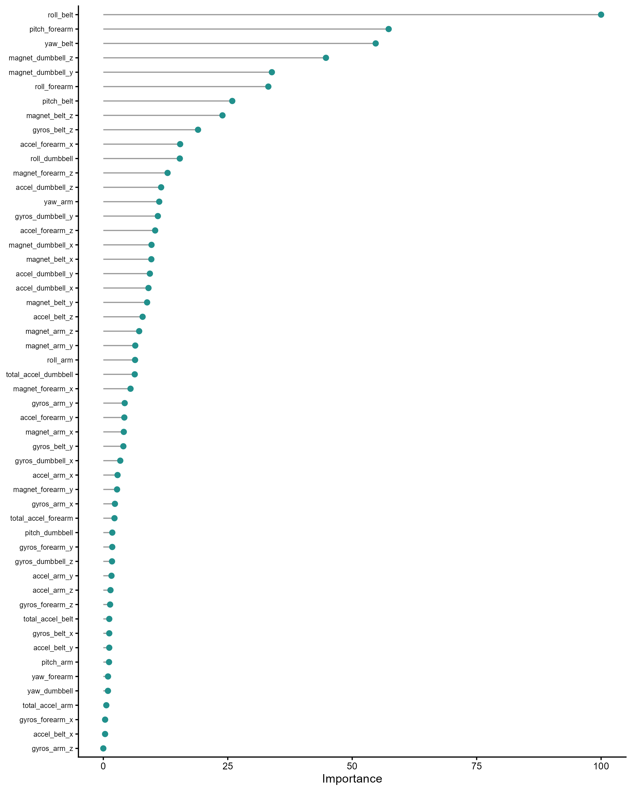
Interpretation: The dominance of belt sensor readings in the GBM mirrors the random forest pattern, reinforcing that core movement signals are the most discriminating features for this classification task regardless of the ensemble method used.

Table 5 shows a similar pattern to the bagged tree – misclassifications distributed across the diagonal with no class collapsing. Table 6 shows sensitivity ranging from 0.938 (Class B) to 0.992 (Class E), with no class falling below the threshold for practical utility. The overall performance gap between GBM and bagging is small enough that the choice between them would depend on computational cost and deployment constraints rather than accuracy alone.

Table 5. Confusion Matrix – GBM

	A	B	C	D	E
A	2185	36	4	7	0
B	49	1433	30	2	4
C	0	43	1307	15	3
D	0	7	37	1238	29
E	2	8	12	4	1391

Table 6. Performance Statistics by Class – GBM

Statistic	A	B	C	D	E
Sensitivity	0.977	0.938	0.940	0.959	0.992
Specificity	0.992	0.987	0.991	0.993	0.992
Pos Pred Value	0.979	0.944	0.955	0.963	0.965
Neg Pred Value	0.991	0.985	0.988	0.992	0.998
Prevalence	0.285	0.195	0.177	0.165	0.179
Detection Rate	0.278	0.183	0.167	0.158	0.177
Detection Prevalence	0.284	0.193	0.174	0.164	0.184
Balanced Accuracy	0.984	0.962	0.965	0.976	0.992

Random Forest: Best Model

The random forest achieved the highest overall accuracy at 99.4% (95% CI: 99.2–99.5%, Kappa: 0.992). Figure 3 shows roll_belt as the dominant predictor by a wide margin, with pitch_forearm and yaw_belt following. The top predictors are concentrated in belt and forearm sensors, with arm and dumbbell sensors contributing far less – suggesting a reduced sensor deployment focused on these locations may be sufficient for accurate classification.

Figure 3. Variable Importance – Random Forest

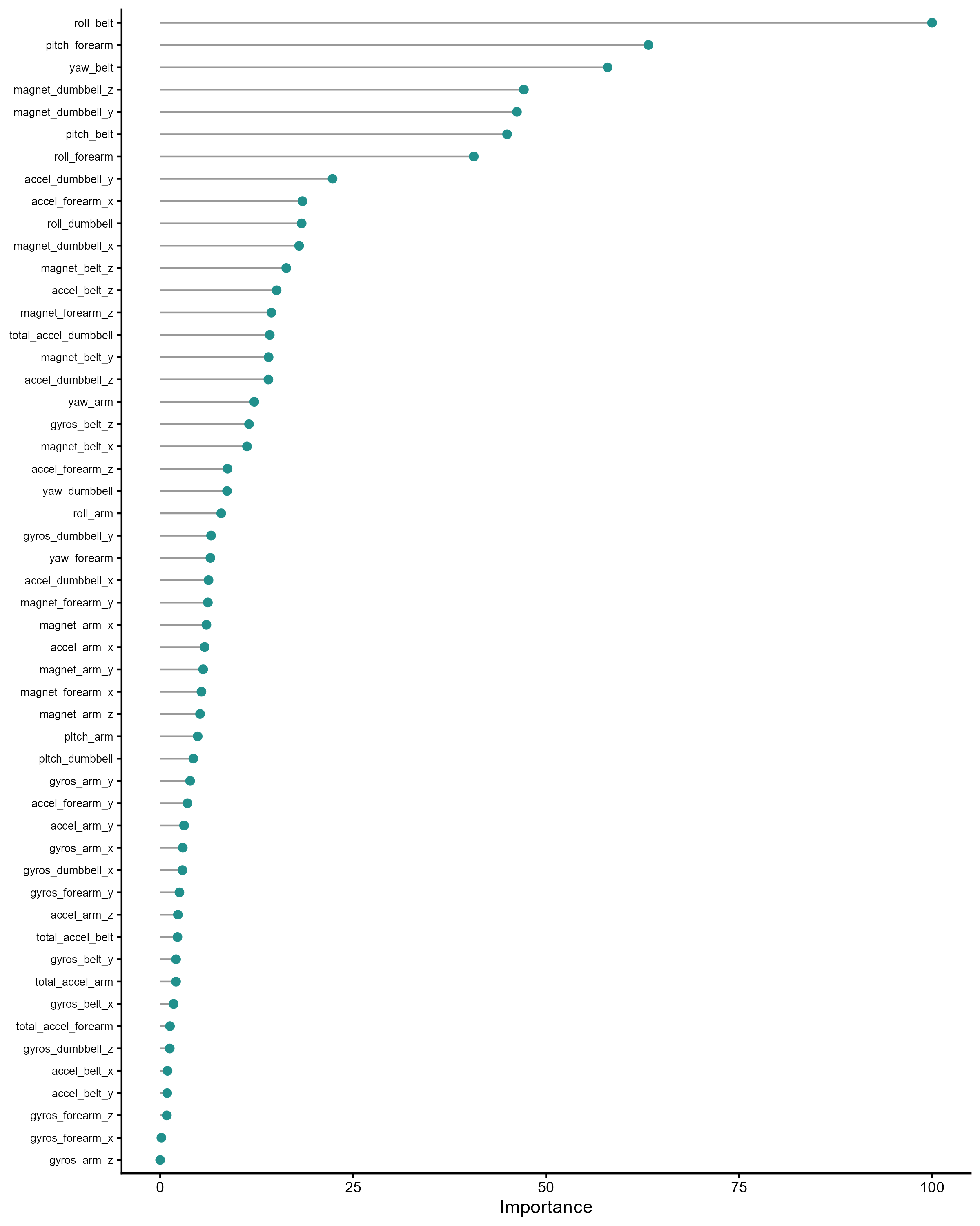
Interpretation: The steep drop-off in importance after the top three predictors – roll_belt, pitch_forearm, yaw_belt – suggests that a substantially reduced predictor set could be used in a leaner deployment model without meaningful loss of accuracy.

Table 7 shows near-perfect classification across all five classes – the entire off-diagonal contains only 71 misclassifications out of 7,846 observations. Table 8 confirms sensitivity above 0.989 for all classes, with Class E reaching perfect sensitivity (1.000) – meaning every hip-forward error in the test set was correctly identified.

Table 7. Confusion Matrix – Random Forest

	A	B	C	D	E
A	2228	3	1	0	0
B	13	1503	2	0	0
C	0	4	1357	7	0
D	0	1	9	1276	0
E	0	0	3	7	1432

Table 8. Performance Statistics by Class – Random Forest

Statistic	A	B	C	D	E
Sensitivity	0.994	0.995	0.989	0.989	1.000
Specificity	0.999	0.998	0.998	0.998	0.998
Pos Pred Value	0.998	0.990	0.992	0.992	0.993
Neg Pred Value	0.998	0.999	0.998	0.998	1.000
Prevalence	0.286	0.193	0.175	0.164	0.183
Detection Rate	0.284	0.192	0.173	0.163	0.183
Detection Prevalence	0.284	0.193	0.174	0.164	0.184
Balanced Accuracy	0.997	0.996	0.994	0.994	0.999

Figure 4 shows how model error evolves as trees are added. All six lines – one per class plus overall OOB error – decline rapidly through the first 50 trees and stabilize around 200, confirming convergence well before the 500-tree maximum. Classes C and D show the highest residual error, consistent with their being the most biomechanically similar form categories.

Figure 4. Model Error by Number of Trees – Random Forest

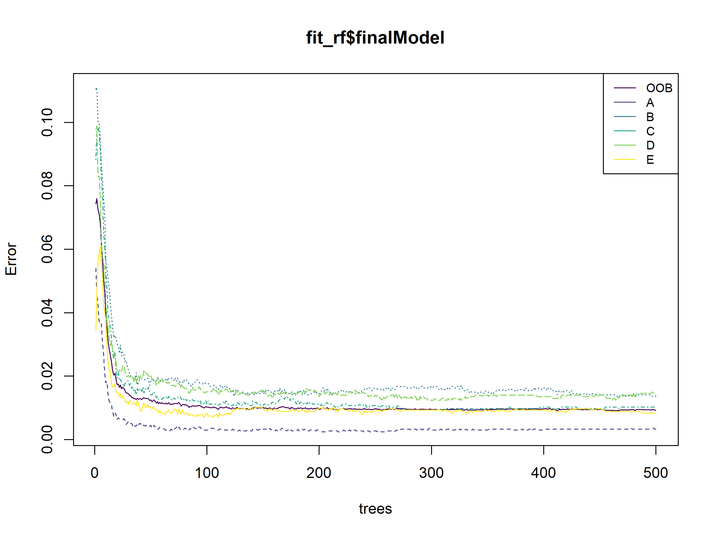
Interpretation: Convergence by ~200 trees means a smaller forest could be deployed in a production setting without sacrificing accuracy. Classes C and D – halfway up and halfway down – remain the hardest to distinguish, which makes biomechanical sense given their similar partial-range-of-motion profiles.

Figure 5 plots cross-validation accuracy across the three predictor subset sizes tested during model tuning. Accuracy is identical at 2 and 27 predictors, then drops sharply at 52, indicating the model does not benefit from the full predictor set.

Figure 5. Model Accuracy by Number of Predictors – Random Forest

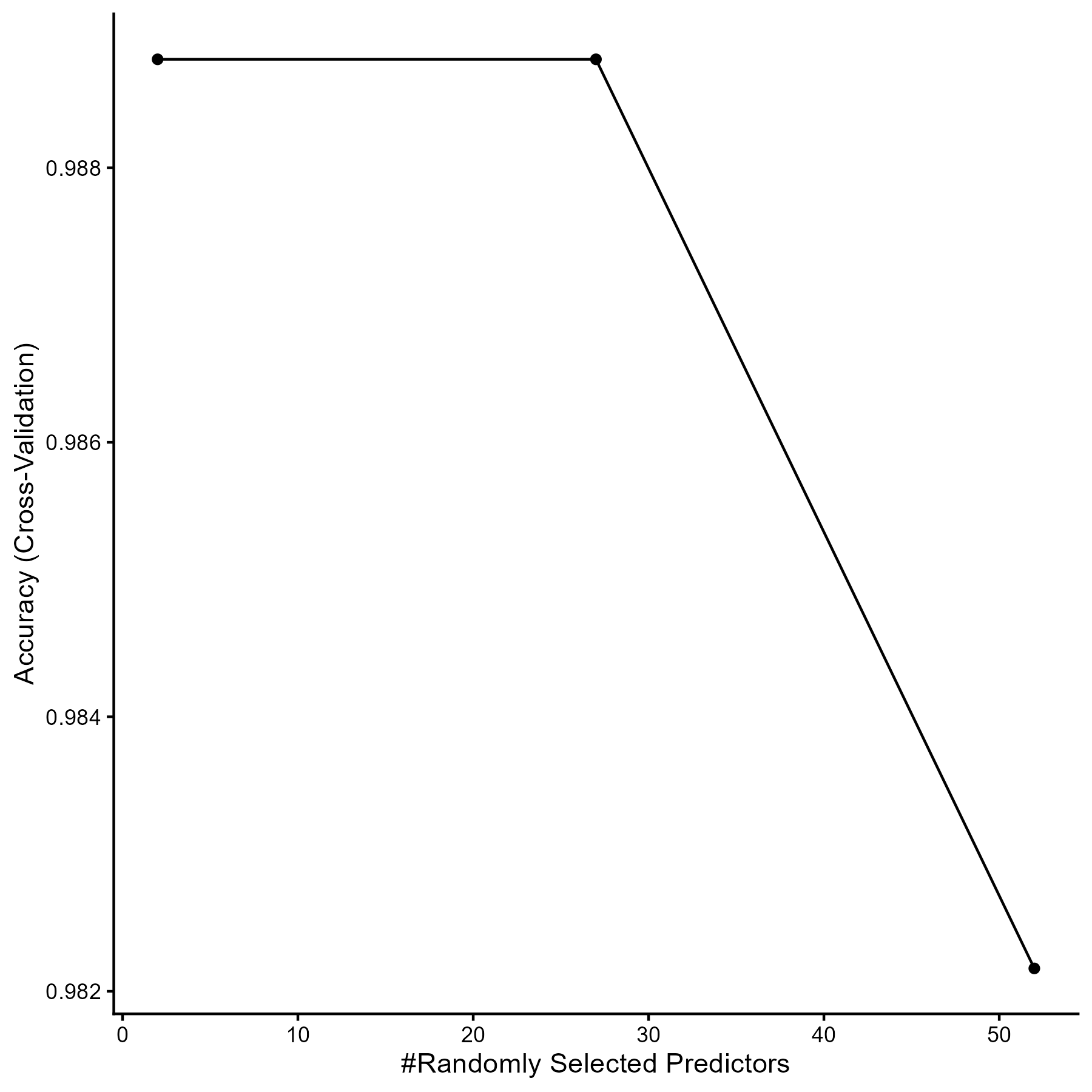
Interpretation: The decline at 52 predictors points to collinearity in the full feature set. A formal collinearity analysis before deployment would identify which predictors are redundant and allow construction of a leaner, more interpretable model.

Model Comparison

Across all four models, the progression from single tree to ensemble methods tells a consistent story: resampling is essential for this classification task, and the random forest outperforms gradient boosting when both are applied to the same data. Table 9 summarizes performance across all four models.

Table 9. Model Performance Summary

Model	Accuracy	95% CI	Kappa	OOS Error
Decision Tree (rpart)	49.7%	48.6–50.9%	0.343	50.3%
Bagged Tree	95.8%	95.4–96.3%	0.947	4.2%
GBM	96.3%	95.8–96.7%	0.953	3.7%
Random Forest	99.4%	99.2–99.5%	0.992	0.6%

The 49.7-percentage-point gap between the decision tree and the random forest is not a marginal improvement – it is the difference between a model that cannot be deployed and one that can. The bagged tree and GBM both represent viable intermediate options, but the random forest’s sub-1% out-of-sample error makes it the clear choice for any real-world application.

Next Steps

Feature reduction: Conduct a collinearity analysis on the 52 predictors. Collinear variables can inflate apparent accuracy; weighting or removing them would produce a leaner, more honest model.
Sensor minimization: Examine whether the top-ranked predictors cluster on specific body locations. If so, a simpler single-sensor or dual-sensor deployment may be sufficient for reliable classification.
Domain validation: Collaborate with an exercise physiologist to evaluate whether the most important predictors correspond to biomechanically meaningful movement signals or are sensor artifacts.
Deployment testing: Evaluate whether accuracy holds under real-world conditions – varied populations, fatigue, different dumbbell weights – before considering integration into consumer fitness technology.

Study Design

Data Source: The Weight Lifting Exercise Dataset was collected by Velloso et al. (2013) as part of the Human Activity Recognition project at the Pontifical Catholic University of Rio de Janeiro. Sensors were strapped to participants’ belts, forearms, upper arms, and dumbbells during supervised bicep curl sessions. Participants performed the exercise in one correct form and four defined incorrect forms under expert supervision. Training and test datasets are publicly available.

Data Handling: Variables unrelated to exercise performance (participant ID, timestamps, window metadata) were removed from both training and test sets. Variables with high proportions of missing values were excluded, leaving 52 predictors from the original feature set. The outcome variable (classe) identifies form category: A (correct), B (elbows forward), C (halfway up), D (halfway down), E (hips forward).

Analytical Approach:

Data partitioned 60/40 into training and test sets using stratified random sampling on classe.
Four models trained using the caret package with 5-fold cross-validation via trainControl: decision tree (rpart), bagged decision tree (bag), gradient boosted random forest (gbm), and random forest (rf).
Each model evaluated on the held-out test set using confusionMatrix: overall accuracy, Kappa, and per-class sensitivity and specificity.
Variable importance extracted for all models to identify top predictors.
Random forest accuracy evaluated across predictor counts (2 to 52) to identify the optimal predictor subset.

Project Resources

Repository: github.com/kchoover14/ml-lift-better

Data: Training and test datasets from the Weight Lifting Exercise Dataset (Velloso et al., 2013), publicly available. Stored in data/.

Code:

scripts/ml-lift-better.R – data cleaning, partitioning, model training, figure export, and table export for all four classifiers

Project Artifacts:

Figures (n=5): variable importance plots for bag, GBM, and random forest; random forest error by tree count; random forest accuracy by predictor count. Stored in outputs/.
Tables (n=9): confusion matrices and per-class statistics for all four models; model comparison summary. Stored in outputs/.

Environment:

renv.lock and renv/ – restore with renv::restore()

License:

Tools & Technologies

Languages: R

Tools: caret | renv

Expertise

Domain Expertise: machine learning | classification | ensemble methods | wearable sensor data | model evaluation

Transferable Expertise: Demonstrates ability to select and compare competing model types, diagnose failure modes in underperforming algorithms, and translate classification results into actionable deployment recommendations for applied technology contexts.